These are some of the most common machine-learning interview questions.
Watch a Snapchat MLE answer common ML interview questions.
Top Machine Learning Interview Questions
Let's cut to the chase.
According to candidates, these are ten of the most frequently asked ML interview questions.
- Explain gradient descent. (OpenAI)
- Explain linear and logistic regression regression. (Amazon)
- Design an evaluation framework. (Meta)
- Design a recommendation system. (Spotify)
- Design a monitoring system.
- Implement k-means.
- Design a detection system.
- Implement a 2D convolutional filter.
- How do you handle an exploding gradient?
- How do you stay up to date with advancements in machine learning?
ML Conceptual Questions
In these interviews, you'll be tested on your understanding of fundamental machine learning and statistical concepts.
These may also be called:
- ML technical assessment interview,
- ML theory interview,
- ML knowledge interview.
There are four categories of questions you should prepare for:
1. What is overfitting? How can you avoid it?
Overfitting happens when a model learns specific details and noise in the training data.

This leads to the model performing well on the training set but struggling to generalize on unseen data.
Good accuracy on training data but poor performance on unseen data is a sign of overfitting.
Data splitting, regularization techniques like L1 and L2 regularization, data augmentation, model fine-tuning, and early stopping are some approaches to prevent overfitting.
2. Explain the bias-variance tradeoff.
- Bias is an error produced by a machine learning model.
- Variance is a model's sensitivity to training data.
There's often a tradeoff between bias and variance due to:
- Simpler models tend to have a higher bias. They might not capture finer details in a dataset.
- Complex models may become too focused on training data, which results in overfitting.
Dataset splitting, appropriate model selection, and regularization techniques help balance the bias and variance.
3. What is hyperparameter tuning?
Hyperparameters control the model learning process and impact model performance. Hyperparameter tuning is finding the right mix of hyperparameters to achieve good performance.
Some common examples of hyperparameters include:
- Train-test split,
- Activation function,
- Hidden layers.
Best practices:
- Using a validation set,
- cross-validation,
- grid or random search,
- model performance analysis,
- and comparison.
4. How do you handle missing or corrupted data in a dataset? Mention some imputation techniques.
Handling missing or corrupted data begins with identifying missing values in a dataset.
There are two broad strategies for handling missing data:
- data deletion
- data imputation
Some imputation techniques are:
- Mean/Median/Mode Imputation: Imputing missing values with the column's mean/median/mode. This technique is simple but can introduce bias.
- KNN Imputation: This method uses the K Nearest Neighbors algorithm to find the closest samples in the training dataset and impute the mean value of those K samples.
- Iterative Imputation: Predicting missing values based on the available data using an iterative approach for better estimation.
5. Explain a confusion matrix.
A confusion matrix evaluates the performance of classification algorithms. It consists of rows and columns representing the actual and predicted classes.
Each cell represents the following:
- True Positive (TP): Correctly predicted positive cases.
- True Negative (TN): Correctly predicted negative cases.
- False Positive (FP): Incorrectly predicted positive cases (Type I error).
- False Negative (FN): Incorrectly predicted negative cases (Type II error).
These instances help measure the accuracy, precision, recall, and F1 score evaluation metrics to assess model performance.
These metrics:
- Ensure an accurate representation of a model's performance,
- Give insights into error types produced by a model,
- And guide toward a tradeoff between precision and recall.
6. What are false positives and false negatives?
A false positive is an error when a model classifies a negative class as positive.
For example, classifying a non-spam email as spam.

A false negative is an error when a model classifies a positive class as negative, such as classifying a spam email as non-spam.
The confusion matrix helps identify the proportion of these errors during model evaluation.
7. How do you pick a suitable machine learning algorithm for your problems?
Choosing the right machine learning algorithms requires:
- Understanding the problem and analyzing data format. Is it a classification, regression, or clustering task? What are the dataset size, format, linearity, and quality?
- Speed and accuracy thresholds.
- Picking multiple algorithms based on your findings.
- Performing cross-validation to avoid overfitting and evaluate model performance.
- Comparing model performance and choosing the best one.
8. Explain principal component analysis (PCA) and its significance.
PCA is an important technique for dimensionality reduction.
It generates important features for model training called principal components (PC). The process begins with standardizing the data and finding a covariance between features.
Using the covariance matrix, PCA calculates the eigenvectors and eigenvalues representing the data's direction and magnitude. Lastly, it sorts the values into descending order, with the highest eigenvalues representing the most important features.
PCA improves model performance and reduces computational costs by reducing the dimensionality of data. It can also visualize high-dimensional data by projecting it into smaller spaces.
9. Explain the architecture of CNN.
Convolutional Neural Network (CNN) is a deep learning architecture for computer vision tasks.
A typical CNN architecture includes:
- Input layers: Receive raw input as vectors representing an image.
- Convolutional layers: These layers apply filters to extract image features, such as edges, shapes, and colors. They also produce feature maps that highlight the presence of features in the image.
- Pooling layers: Reduce the dimensionality of feature maps using techniques like average pooling and max pooling.
- Activation layers: Introduce non-linearity in the network to learn complex patterns.
- Fully connected layer(s): Connect neurons from the previous layers to every neuron in this layer and classify the input into target labels.
- Output layer: Produces the final output depending on the task.
10. Explain batch, mini-batch, and stochastic gradient descent.
Gradient descent is an optimization technique calculated by taking the derivative of loss with respect to algorithm parameters.
Gradient descent represents the direction of the steepest descent; it can be used to take gradual steps toward the minimum of that loss function.
- Batch gradient descent: Uses the entire training set in one go. You compute the gradient, then do a single gradient descent step.
- Mini-batch gradient descent: Divides the training set into mini-batches and typically chooses a batch size. Gradients are separately computed on mini-batches. After that, you'll move a step in that direction for each mini-batch.
- Stochastic gradient descent: Related to both batch and mini-batch gradient descent, but mostly refers to shuffling up the training set randomly. Similarly, you would divide that up into smaller batches, compute the gradients on those batches, and perform the respective parameter updates.
11. Describe precision, recall, and F1-score. When would you use each?
This question is meant to help evaluate the performance of a machine-learning model.
- Precision: Measures the proportion of predicted positive cases that are actually correct. Precision is crucial when the cost of misclassifying a negative case as positive is high, like in spam filtering or healthcare.
- Recall: Measures the proportion of actual positive cases correctly identified by your model. Recall is crucial when missing positive cases is costly, like misdiagnosing a disease.
- F1-score: A harmonic mean of precision and recall representing the model's overall performance by balancing the two metrics. It's beneficial when dealing with imbalanced datasets where one class is significantly higher in number than the other.
12. What is the difference between one hot encoding and label encoding?
- One-hot encoding: This method represents categorical features as binary vectors, increasing the dimensionality of the data. It treats all categories equally and independently. It suits algorithms that work well with numerical features and can handle higher dimensionality.
- Label encoding: Assigns an integer to each category in the variable. It maintains the dimensionality of data but can introduce bias if a model interprets numerical values as ordinal.
13. How do you ensure data quality in ML tasks?
- Data acquisition from reliable sources and understanding its origin, format, and features.
- Handle missing data points, addressing inconsistencies and outliers in input data.
- Understand data distribution and explore patterns.
- Standardize/normalize features and feature engineering to improve model performance by using important input features.
- Split data into validation and test sets to assess model performance on unseen data. Use a cross-validation score to measure the model's generalizability.
- Track model performance and analyze errors to understand potential bias.
14. Explain classification vs. regression.
Classification and regression refer to the type of outcome predicted by a supervised algorithm.
Classification predicts some categories, like Yes/No or Hot/Cold.
Regression predicts numerical or continuous values such as a person's height.

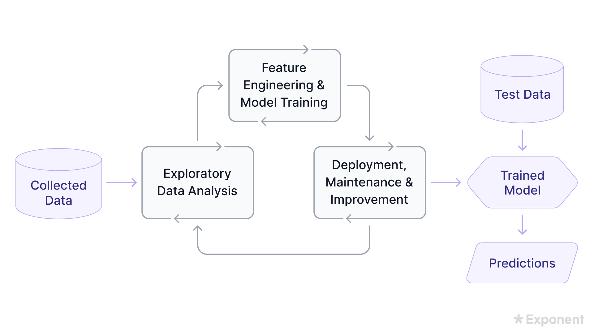
15. Explain the lifecycle of a machine learning application.
The machine learning lifecycle is a process of building, deploying, and maintaining machine learning applications.
The key stages include:
- Problem definition, motivation, and business understanding.
- Data acquisition and exploration.
- Data cleansing and preprocessing to prepare it for machine learning.
- Appropriate model selection and training.
- Model evaluation on unseen data and identification of bias and errors.
- Model deployment for real-world use and monitoring its performance.
- Iterative model refinement based on monitoring and user feedback.
16. Explain the concept of dropout in neural networks.
Dropout is a regularization technique for preventing model overfitting.
It randomly drops neurons during the training to force the network to learn other features without depending on other neurons.
Dropout enhances a model's generalization ability on unseen data and improves its robustness.
17. How does batch normalization work? What are its benefits?
Batch normalization addresses the internal covariate shifts, which can hinder learning.
It works by calculating the mean and standard deviation of the activations for each network layer in each mini-batch.
It then standardizes the activations and introduces gamma (scale) and beta (shift) to avoid losing information during standardization.
Batch normalization offers faster convergence, reduced sensitivity, and higher learning rates.
18. How do you handle an imbalanced dataset?
Handling imbalanced datasets starts with picking the evaluation metrics.
Using the SMOTE method ensures that the model is not repeatedly trained on the same data, which helps handle data imbalance.
F1 score is generally a suitable metric for imbalanced datasets since it represents the harmonic mean of recall and precision.
Oversampling and undersampling help balance the minority or majority class with the other.
Undersampling can be done by deleting the majority class, and oversampling can be achieved through the SMOTE algorithm.
Another technique, a balanced bagging classifier, is an ensemble learning method that uses random undersampling to balance the class distribution in each subset.
Threshold moving is another technique that involves changing the threshold so that the model efficiently separates the two classes.
19. What are the different types of machine learning?
The three fundamental types of machine learning are:
- Supervised learning: This method uses labeled training data to learn patterns in data, such as email spam filtering or animal breed classification.
- Unsupervised learning: Unlabeled data detect hidden patterns without guidance, e.g., clustering or dimensionality reduction.
- Reinforcement learning: Uses the trial and error method to learn patterns where the model is penalized for every incorrect prediction and detects hidden details iteratively, e.g., self-driving cars.
Semi-supervised learning uses a combination of labeled and unlabeled data.
Labeled data guides the model toward learning data patterns, and unlabeled data improves model generalizability.
Deep learning is a subfield of machine learning that uses neural networks to detect complex patterns. It is used in chatbots and image classification.
20. Explain "training" and "testing" data.
Training data refers to the portion of the data that a machine learning algorithm uses to learn patterns.
The test set is the unseen data portion used to assess the algorithm's performance.
21. What is a recommendation system? How does it work?
A recommendation system is a machine learning application that analyzes user data and filters items (products, movies, songs, etc.) to suggest items to users based on their preferences.
It gathers user data, including interactions, browsing history, purchase history, ratings, and reviews, to capture user preferences.
Additionally, collaborative and content-based filtering creates user profiles to capture individual preferences.
Collaborative filtering identifies users with similar tastes and recommends items they like. Content-based filtering identifies items similar to the user's past interactions.
A recommendation system generates personalized recommendations based on these identifications and user profiles.
22. What is the curse of dimensionality?
The curse of dimensionality refers to the issues caused by high-dimensional data in machine learning.
High-dimensional data introduces the challenge of data sparsity, meaning that most of the high-dimensional space is empty.
Visualizing and degrading the performance of algorithms that rely on distance, like k-nearest neighbors, is difficult.
Also, models tend to overfit high-dimensional data and are computationally expensive.
23. Explain the support vector machine (SVM).
SVM is a supervised classification algorithm that uses a margin and hyperplane to separate classes.
Hyperplanes are decision boundaries that help classify the data points, with data points closest to the boundary known as support vectors.
The SVM algorithm aims to find the hyperplane with the maximum margin, i.e., the maximum distance between the classes.

24. What is the difference between random forests and decision trees?
Both random forests and decision trees are supervised models for classification and regression tasks.
They rely on a tree-like structure representing feature rules that map to the target label.
The decision tree builds a single tree on the training dataset and considers all features at each split. Random forests are an ensemble learning technique that builds various trees on random subsets of data.
- Decision trees are more prone to overfitting and can be sensitive to data changes.
- Random forests are less prone to overfitting and more generalizable.
25. Explain ETL.
ETL stands for Extract, Transform, and Load.
- Extract: Data from various sources such as transactional databases, spreadsheets, flat files, and external APIs.
- Transform: Clean, format, and transform data to ensure consistency and compatibility.
- Load: Load the transformed data into your target system to analyze and make informed decisions.
ML Coding Questions
Machine learning coding questions will test your familiarity with ML frameworks (e.g., TensorFlow, PyTorch) and core ML concepts relevant to the team's sub-field.
Expect questions like:
- Implement an attention mechanism using PyTorch.
- Implement a convolutional filter using TensorFlow.
- Implement k-means clustering.
- Find the common ancestors in a tree.
- Implement a depth-first search algorithm.
An effective ML coding interview answer follows these steps:
- Step 1: Understand the problem. Ask clarifying questions, try a few toy examples, and ensure you understand the inputs and outputs. (5-7 minutes)
- Step 2: Discuss the approach. Write out a high-level outline of your algorithm in pseudo-code. Get buy-in or approval from the interviewer. (3-5 minutes)
- Step 3: Implement the algorithm. Decide on a particular ML framework (e.g., PyTorch or TensorFlow) and language (usually Python). Implement the algorithm, and talk out loud as you write the code. (20-25 minutes)
- Step 4: Test the code and discuss the results. Test your code, discuss the results, and note any significant takeaways. Check back in with the interviewer about any follow-up questions. (7-8 minutes)
1. Pre-process a dataset for a machine learning task.
Here, you're being assessed on your ability to preprocess data in a machine-learning pipeline and identify opportunities for feature manipulation and extraction.
This is a pseudo code solution using sklearn:
import pandas as pd
from sklearn.impute import SimpleImputer
from sklearn.preprocessing import LabelEncoder, StandardScaler

# Load the dataset
data = pd.read_csv("data.csv")

# Check for missing values
print(data.isnull().sum())  # This shows the number of missing values per column

# Handle missing values (choose one approach)
# Option 1: Remove rows with missing values
# data.dropna(inplace=True)

# Option 2: Impute missing values (e.g. with mean/median)
imputer = SimpleImputer(strategy="mean")  # You can choose other strategies
data = pd.DataFrame(imputer.fit_transform(data))

# Encode categorical features (if any)
categorical_cols = [col for col in data.columns if data[col].dtype == object]
le = LabelEncoder()
for col in categorical_cols:
    data[col] = le.fit_transform(data[col])

# Feature scaling (optional, depends on the algorithm)
scaler = StandardScaler()
numerical_cols = [col for col in data.columns if data[col].dtype != object]
data[numerical_cols] = scaler.fit_transform(data[numerical_cols])

# Split data into training and testing sets (assuming labels are in a separate column)
X = data.drop("target_column", axis=1)  # Replace "target_column" with your actual label column name
y = data["target_column"]

from sklearn.model_selection import train_test_split
X_train, X_test, y_train, y_test = train_test_split(X, y, test_size=0.2, random_state=42)

# Now you have your preprocessed data split into training and testing sets
print(X_train.shape, X_test.shape, y_train.shape, y_test.shape)
2. Evaluate the performance of a machine learning model on a held-out test set.
Can you evaluate the performance of a model and pick the right metrics?
This is a pseudo code solution using sklearn:
from sklearn.model_selection import train_test_split
from sklearn.metrics import accuracy_score, precision_score, recall_score, f1_score
from sklearn.linear_model import LogisticRegression

# Load and preprocess data

# Split data into training and testing sets (70/30 split here)
X_train, X_test, y_train, y_test = train_test_split(X, y, test_size=0.3, random_state=42)

# Train your machine learning model (replace with your model training logic)
model = LogisticRegression()
model.fit(X_train, y_train)

# Make predictions on the test set
y_pred = model.predict(X_test)

# Evaluate the model performance
accuracy = accuracy_score(y_test, y_pred)
precision = precision_score(y_test, y_pred)
recall = recall_score(y_test, y_pred)
f1 = f1_score(y_test, y_pred)

print("Accuracy:", accuracy)
print("Precision:", precision)
print("Recall:", recall)
print("F1-score:", f1)
3. Fine-tune a pre-trained deep learning model on a new dataset.
Fine-tuning involves modifying a pre-trained model based on your project requirements, demonstrating your practical understanding of adjusting a model to suit specific needs.
This is a pseudo code solution using Tensorflow:
from tensorflow.keras.applications import VGG16  # Replace with your pre-trained model
from tensorflow.keras.layers import Flatten, Dense
from tensorflow.keras.models import Model

# Load the pre-trained model (exclude the top layers)
base_model = VGG16(weights="imagenet", include_top=False, input_shape=(img_height, img_width, 3))  # Adjust for your image data

# Freeze the base model layers (optional, adjust freezing strategy)
for layer in base_model.layers:
    layer.trainable = False  # You can freeze specific layers instead of all

# Add new layers for fine-tuning
x = base_model.output
x = Flatten()(x)
x = Dense(1024, activation="relu")(x)  # Adjust number of units and activation as needed
predictions = Dense(num_classes, activation="softmax")(x)  # Replace num_classes with your actual number of classes

# Create the final fine-tuned model
model = Model(inputs=base_model.input, outputs=predictions)

# Compile the model (adjust optimizer and loss based on your task)
model.compile(optimizer="adam", loss="categorical_crossentropy", metrics=["accuracy"])

# Load and pre-process your new dataset
# Train the model on the new dataset
# Adjust epochs and batch size

# Evaluate the model on the validation set
4. Code a linear regression model.
The hands-on assessment will offer insight into your coding skills, attention to detail, and communication skills when you present your solution.
This is a pseudo code solution using sklearn:
from sklearn.linear_model import LinearRegression
from sklearn.model_selection import cross_val_score, train_test_split

# Example usage (replace with your data loading and preprocessing)
# X_train, X_test, y_train, y_test = your data loading and splitting logic

# Create the linear regression model
lr = LinearRegression()

# Train the linear regression model
model = lr.fit(X_train, y_train)

# Make predictions on the test set
y_pred = lr.predict(X_test)

# Evaluate the model performance (replace with your chosen metrics)
scores = cross_val_score(lr, X_train, y_train, cv=5)
mean_accuracy_score = scores.mean()
print("Accuracy score of each fold:", scores)
print("Mean accuracy score:", mean_accuracy_score)
5. Implement K-means clustering.
K-means clustering is a fundamental unsupervised learning algorithm for partitioning a given dataset into K distinct, non-overlapping subsets (clusters).
The goal is to determine the best way to group data points into clusters based on their similarity.
A key part of this algorithm involves calculating the Euclidean distance between points to measure similarity.
This is a pseudo code solution using numpy:
import numpy as np

class Centroid:
    def __init__(self, location, vectors):
        self.location = location  # (D)
        self.vectors = vectors    # (N_i, D)

class KMeans:
    def __init__(self, n_features, k):
        self.n_features = n_features
        self.centroids = [
            Centroid(
                location=np.random.randn(n_features),
                vectors=np.empty((0, n_features))
            )
            for _ in range(k)
        ]

    def distance(self, x, y):
        return np.sqrt(np.dot(x - y, x - y))

    def fit(self, X, n_iterations):
        for _ in range(n_iterations):
            # start initialization over again
            for centroid in self.centroids:
                centroid.vectors = np.empty((0, self.n_features))

            for x_i in X:
                distances = [
                    self.distance(x_i, centroid.location) for centroid in self.centroids
                ]
                min_idx = distances.index(min(distances))
                cur_vectors = self.centroids[min_idx].vectors
                self.centroids[min_idx].vectors = np.vstack((cur_vectors, x_i))

            for centroid in self.centroids:
                if centroid.vectors.size > 0:
                    centroid.location = np.mean(centroid.vectors, axis=0)

    def predict(self, x):
        distances = [self.distance(x, centroid.location) for centroid in self.centroids]
        return distances.index(min(distances))
6. Split a dataset into training, evaluation, and testing sets.
Decide the training, evaluation, and testing set size based on the dataset size.
from sklearn.model_selection import train_test_split

# X = your features (data)
# y = your target labels

# Splitting with a dedicated evaluation (validation) set
X_train, X_test_val, y_train, y_test_val = train_test_split(X, y, test_size=0.2, random_state=42)

# Further split the test/validation set into testing and validation (optional)
X_test, X_val, y_test, y_val = train_test_split(X_test_val, y_test_val, test_size=0.5, random_state=42)
ML System Design Questions
ML system design questions are more specific to your ML background.
Most machine learning system design interviews include discussions of data, models and frameworks, and scaling. You'll be evaluated on your ability to clearly communicate your ideas.
Questions might focus on pre-processing data, training and evaluating a model, and deploying a model.
Expect questions on real-world use cases like efficiency, monitoring, preventing harmful model outputs, and building inference infrastructure.
Ask clarifying questions like input/output assumptions, the scope of the question, and acceptable tradeoffs.
Craft a high-level design of the system and relate infrastructure questions back to foundational ML concepts.
If you're interviewing at a large company, prepare to respond to follow-up questions about how you'd scale the system.
1. How do you approach machine learning system design problems?
The ML system design formula includes:
- Problem Formulation: Begin by understanding the type of ML task, its requirements, and assumptions. Identify the business goal, required features, data sources, prediction latency, and other key factors.
- Identifying Metrics: Choose metrics that showcase model performance. Consider precision, recall, F1 score, ROC AUC, P/R AUC, mAP, and log-loss for classification. For regression tasks, metrics like MSE (Mean Squared Error) and MAE (Mean Absolute Error) are essential.
- Building MVP Logic: Conceptualize the high-level architecture and main components, including the user application, server, databases, knowledge graphs, and interactions.
- Data Collection: This stage collects data based on factors like cost, availability, and type. It also involves preparing and transforming raw data into useful information.
- Feature Engineering: Select the right features, perform feature transformations, and normalize data to enhance model performance.
- Model Development and Evaluation: Select a model appropriate for the task’s complexity and requirements. Train the model on preprocessed data and evaluate it on unseen data to gauge its applicability.
- Testing: Rigorously test the model to ensure its robustness and reliability before deployment.
- Deployment: Deploy the model for end-users, ensuring it integrates seamlessly with existing systems and workflows.
- Monitoring: Continuously monitor the deployed model to track potential risks and make timely improvements.
2. What are the architectural components in ML system design?
The core components of an ML system design architecture are:
- Data acquisition
- Data storage
- Model training and evaluation
- Model deployment
- Monitoring
- Feedback
Security, privacy, and scalability are additional features to consider throughout the ML lifecycle.
3. Design a recommendation system for Spotify.
Your answer will reveal your ability to develop practical ML solutions.
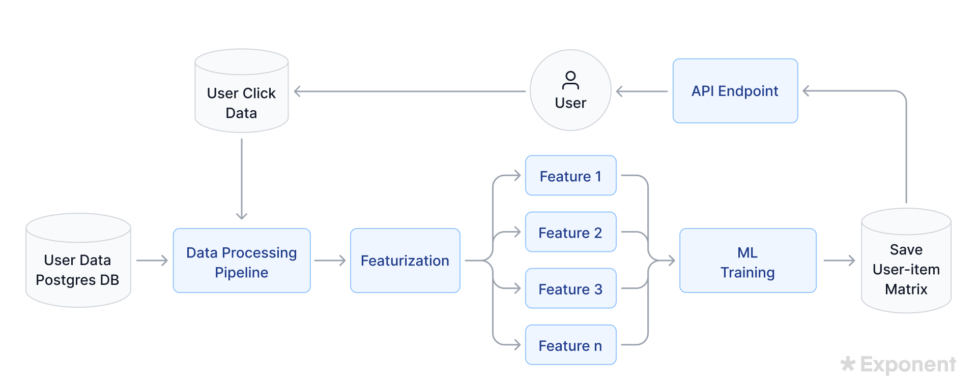
Solution:
Step 1: Define the problem
Spotify's recommendation system success relies on user engagement, measured by click numbers.
We assume click data as one data source and user metadata (age group, location, previous info) as another.
Click data is JSON format, and user metadata is in a Postgres account table.
Handling Personally Identifiable Information (PII) with care is essential.
Step 2: Design the data processing pipeline
To collect and process data, choose between batch-based or real-time solutions.
Batch-based systems are easier to manage, while real-time processing is compute-intensive and costly.
Training and inferencing will be batch-based, with serverless jobs updating recommendations in a cache every few hours.
Click data in JSON format lands in an object store, so we'll design an ETL pipeline and create an abstracted data model.
Feature Engineering Steps:
- Read and De-serialize Data: Convert raw data into a usable format.
- Extract Features: Derive age group (masking PII), parse location, and extract details for the most recent 100 favorite artists and last 100 listened songs.
- Clean and Transform Data: Lowercase text, remove spaces, punctuation, noise, de-duplicate entries, and format timestamps.
- Load Features to Database: Store cleaned features in a Postgres table.
- Export Features to Feature Store: Send features from the database to a dedicated feature store for model consumption.
Step 3: Model architecture
Recommendation systems use data from other users to suggest items. We'll create feature vectors for each user, combining their features (age group, location, favorite artists, and songs). Each feature vector score ranges from -1 to 1, normalizing scores for comparison.
We'll organize these scores into a user-item matrix and compute the product of each feature vector's score with the recommended song's score. A threshold between -1 and 1 determines if an item is recommended, starting with a low threshold to gather information and later optimizing it.
Train and Evaluate the Model
- Training Inputs: Process data, code non-numerical data, and feature the rest.
- Training Output: A user-item matrix for probabilistic predictions as recommendations.
- Evaluation: Collect user clicks as positive feedback. The click ratio over total recommendations measures model accuracy.
Analyzing feature differences between positive and negative recommendations helps create a feature weighting algorithm.
Step 4: Deploy the model
Define engagement metrics and deploy an A/B test plan to assess user experience improvements.
Use AWS SageMaker, Lambda, and Elasticache for training, testing, requesting recommendations, and storage.
4. Explain how you would ensure high availability and fault tolerance in a machine learning system for real-time fraud detection.
Real-time fraud detection systems require high availability and fault tolerance to ensure continuous protection and security.
The strategies that ensure high availability and fault tolerance are:
- Distributed architecture: Redundant components allow systems to function even when some components fail.
- Load balancing: Sharing load across multiple workers prevents workers from overloading and points of failure.
- Redundant data pipelines: Multiple data pipelines ensure continuous data flow even if a pipeline fails.
- Data duplication: Duplicate training data across servers so that others can continue the transaction if a server fails.
- Model redundancy: Duplicate the model across various servers so that the system continues to function if a server fails.
- Health monitoring: Continuously monitor the system's health and implement automatic failover mechanisms so that if a failure happens, the system can switch to healthy backups.
- Error detection: Implement detection mechanisms to detect errors during data processing or model predictions to handle errors on time.
- Alerting and notification: Implement an alerting and notification system to stay updated with system performance.
5. How is data collected, stored, and preprocessed before being fed into ML models?
- Data collection: Identify data sources that depend on your problem, such as databases, APIs, sensors, web scraping, user interaction, etc. Combine data from all the sources into a unified format, including inconsistencies or duplicates during the merging process. This also involves schema mapping and data transformation.
- Data storage: Choose the proper data storage, such as a data lake for storing unstructured data, a data warehouse for structured data, or a feature store for storing machine learning model features, etc. Organize data to facilitate data retrieval and analysis and implement security measures to ensure data protection throughout the pipeline.
- Data preprocessing: Clean and preprocess data using techniques like imputation, transformation, and feature engineering to make the data compatible with ML processing. Detect and address outliers to avoid potential bias in prediction.
6. Design an ETA system for Maps.
Ask the following questions to ensure you understand the problem assumptions:
- Is this product intended to work everywhere or in a specific region?
- Can we assume access to low latency resources (e.g., compute nodes, key-value store)?
Step 1: Clarify data acquisition
- Map System 1: Contains road information:
- Distance
- Speed limit
- Free flow speed (fastest typical speed)
- Priority class (e.g., major highway, local road)
- Historical Travel Data System 3: Contains travel information:
- For each (segment, 2-minute interval):
- Number of cars
- Average speed
- For each (segment, 2-minute interval):
The shortest paths functionality finds the shortest path in a weighted graph. No additional labeling is needed.
Step 2: Bridge the problem space and data space
Organize raw data into two tables:
- Table 1 "map_table":
- segment_id (index)
- Distance
- Speed limit
- Free flow speed
- Priority class
- Table 2 "travel_table_1":
- Year (index)
- Interval within the year (index)
- Number of cars
- Average speed
Ensure data tables are >99% correct by removing rows with null or invalid data. Create convenient data repositories using JOIN tables.
- Table 3 "travel_table_2":
- Interval within the week (index)
- Number of cars
- Average speed
Create this downstream table via SQL query or an offline Python data pipeline.
Now, create an online data processing pipeline to compute the mean (ETA) in:
- Table 4 "record_table":
- segment_id
- Interval within the week
- Number of cars (aggregate)
- Average speed (aggregate)
- ETA
These records map (road, time) to ETA for training and validation.
Calculate:
- Overall number of cars: Sum of cars for each interval.
- Overall average speed: Weighted average of all speeds, weighted by the number of cars.
- ETA: Distance divided by the average speed.
Step 3: Parametrize the inference function
Define the interface by defining an inference function:
def f (segment_id, interval_within_week) -> (ETA)Use the same interval per week to confirm weekly patterns in the data.
Step 4: Train learned functions
Train the model using a simple parametrization formula predicting travel time using the historical mean:
ETA = f(segment_id, interval_within_week) = mCompute the historical mean for each (segment_id, interval_within_week) and store it in a dictionary for inference.
Step 5: Validate the overall approach.
Perform an 80-20 train-validation split, randomly selecting 20% of months for validation.
Metrics computation involves:
- Compute
pred_etausing training records up to the metric computation record. - Fetch
true_eta. - Compute the absolute difference between
pred_etaandtrue_eta. - Aggregate metrics to calculate the mean, variance, and interquartile range.
Summarize validation:
- Perform 80-20 train-validation split at the month level.
- Create a model using training records.
- Compute a distance metric on each validation record.
- Compute statistics on those metrics.
Step 6: Deploy the model
During deployment, use all available historical data. Store the function in a high-performance key-value store.
The user application calls an ETA backend using two key components:
- ETA function: Assigns ETAs to nearby road segments.
- Shortest paths functionality: Computes the best path and its ETA.
7. How do you monitor model performance, data quality, and system health?
- Model performance monitoring involves tracking appropriate evaluation metrics and setting up metric thresholds to receive continuous updates about model performance. It also involves model drift detection and tracking to track changes in model performance over time.
- Data quality monitoring: Monitoring how often data is ingested into the system, validating data schemas, and regularly analyzing anomalies and unexpected changes in data distribution.
- System health monitoring involves tracking system resource utilization, such as CPU and bandwidth usage, error rates, and prediction latency. Logging and alerting help capture system events and errors for timely intervention.
ML Behavioral Interview Questions
This round assesses your values, work ethic, and working style.
- Describe your machine-learning experience.
- Tell me about a machine learning project you worked on.
- How do you manage projects under pressure?
- Tell me about trends and challenges in your machine learning specialty.
- Describe a time you overcame a difficult situation.
Prepare answers to common questions like successes, failures, conflicts, and challenges beforehand.
Provide context to the interviewer for each answer to help them understand the situation and clarify what you did, why, and the results you achieved.
FAANG+ ML Interview Questions
This section will discuss some of the most commonly asked questions during interviews at
1. What is the interpretation of the ROC area under the curve?
Receiver operating characteristics (ROC) is a binary classification evaluation tool showing a tradeoff between sensitivity and specificity.
Sensitivity is the probability of a model predicting an outcome as positive when the actual output is also positive. Specificity is the probability of a model predicting an outcome as negative when the actual outcome is negative.
The area under the curve shows the model's performance.
If the area under the ROC curve is 0.5, the model is entirely random.
If the curve is closer to 1, the model performance is good, and vice versa.
2. What are the methods of reducing dimensionality?
Two broad methods of dimensionality reduction are feature selection and feature extraction.
- Feature selection: The process of finding the important features for the prediction. Filter, Wrapper, and Embedded methods help identify important features for better model performance.
- Feature extraction: The process of manipulating existing features to create new features that have a greater impact on prediction. Linear discriminant analysis (LDA) and principal component analysis (PCA) are the most common feature extraction techniques for extracting features without information loss.
3. Design a product recommendation system.
The interviewer wants to assess your understanding of real-world machine learning applications. Begin by clarifying questions like:
- What's the product?
- Is there a certain demographic/location we're targeting?
- What's the goal of the recommendation system?
- Product and target audience: The product is PhotoShare, a mobile photo-sharing app focused on Millennials, Gen Z, and celebrities. We want to ensure granular sharing control and privacy (default share time, temporary photo sharing).
- User requirements and recommendation engine: Photo visibility is based on the sharer-viewer relationship and duration (photos disappear after a certain duration).
- Recommendation strategy: We'll start with a rule-based model and switch to AI once we've data.
The variables for the rule-based model are:
- User's preferred photo type (most interacted with).
- Sharer-viewer closeness.
- Photo's current engagement.
- Photo's freshness/recency.
- User's current mood (optional login prompt).
Variables for AI modeling are:
- Optimize watch time (North Star Metric).
- Utilize the same variables as the rule-based system.
- Train on data collected during the initial phase.
Evaluation metrics: Watch time will be the primary metric. Clicks, comments, likes, DAU, WAU, MAU, weekly retention, 30-day retention, and user engagement are secondary metrics.
A/B Testing: Continuously test and refine the recommendation algorithm using A/B testing to ensure it optimizes user engagement and watch time.
4. What are the different types of activation functions?
The activation function is used to add non-linearity to neural networks.
When the input is passed through the activation function, it decides whether or not a neuron should be activated before passing it to the next layer.
Without an activation function, a neural network is a linear regression model which cannot learn complex patterns.
These are the most common types of activation functions:
- Sigmoid function: Often used for classification problems and outputs a value between 0 and 1. However, it can suffer from the vanishing gradient in deep neural networks.
- Softmax function: Often used for multi-class classification problems and outputs a value between 0 and 1.
- ReLU: Outputs the input if it's positive, otherwise outputs 0. If the weights become negative during training, it can cause some neurons never to fire again, known as dying ReLU.
- Leaky ReLU: Introduces a small positive slope for negative inputs to address the problem of dying ReLU.
5. Explain the vanishing gradient.
Gradients are used to adjust network weights. A vanishing gradient occurs when it becomes too small to train the model. This can result from multiplying gradients with zero or negative weights or activation functions which decrease the outputs in the range of 0-1 for large inputs.
Vanishing gradients result in slow and shallow neural network learning. This prevents the model from learning patterns and disregards the benefits of deep layers.
6. What are the assumptions of linear regression?
The linear regression model maps the relation between dependent and independent values.
The difference between actual and predicted values is known as residuals.
The assumptions of a linear regression model are:
- The residuals are independent.
- There is a linear relation between the independent variable and the dependent variable.
- Constant residual variance at every level of the independent variable.
- The residuals are normally distributed.
7. Explain the difference between linear and logistic regression.
Linear regression predicts numerical values, whereas logistic regression predicts categories.
For example, an e-commerce website pricing recommendation engine is built on a linear regression model where variables like competitor price, internal economics, and consumer demand predict prices.
However, Netflix uses a multiclass logistic regression model to predict the genre of a movie based on features.
8. How would you explain computer vision to your grandmother?
I would explain computer vision to my grandma as: "Do you remember how you taught me alphabet matching?
I tried to memorize that D is for dish and F is for fish. Computers can similarly learn information.
Some algorithms teach computers to recognize differences between different things like a cat and a dog.
So whenever a human asks computers to identify an object in an image, computers give almost accurate answers."
Preparing for ML Interviews
Learn how to prepare for machine learning interviews.
Company Research
Company research gives you an idea of the company culture and expectations before you appear in the interview.
Scanning a company's social media offers insights into their work ethic and interesting ML projects.
Peer mock interviews
Practice coding questions with peers so your Python knowledge feels fresh on the day-of.
You can find numerous coding questions and their solutions online.
Exponent's ML Interview Course
Exponent's machine learning course can help you crack machine learning interviews.
Built with expert MLEs from FAANGs and startups, this course has helped candidates land jobs at Meta, Google, Apple, Netflix, and more.
Read papers
Reading research papers will prepare you for advanced questions related to development in the machine learning domain.
Domain-specific questions are likely in your screening rounds with team leads.
For example, video processing-related papers for Netflix interviews.
FAQs
How do I prepare for a machine learning interview?
Prepare for a machine learning interview by reviewing core ML concepts, coding questions, system design, data science, and behavioral questions.
Practice mock interviews, read research papers, and understand the specific requirements of the company you're applying to.
What are the 4 types of machine learning?
The four types of machine learning are supervised learning, unsupervised learning, semi-supervised learning, and reinforcement learning.
How do I explain an ML project in an interview?
To explain an ML project in an interview, describe the problem you aimed to solve, the dataset used, the model chosen, the evaluation metrics, and the results, including any challenges faced and how you addressed them.
Good luck in your upcoming interviews!
Book time with a Machine Learning Engineer coach
- Mock interviews
- Career coaching
- Resume review
Learn everything you need to ace your machine learning interviews.
Exponent is the fastest-growing tech interview prep platform. Get free interview guides, insider tips, and courses.
Create your free accountRelated Courses

Machine Learning Engineer Interview Prep

SQL Interviews
Related Blog Posts
Machine Learning System Design Interview (2026 Guide)

Complete Guide to Machine Learning Engineering Interviews

How to Become a Machine Learning Engineer
