Top 25 Statistics Data Science Interview Questions in 2024

Statistics questions are a common part of data science interviews.

Interviewers are looking for “unicorns” who have both technical and business communications skills to analyze and discover meaningful insights within a dataset.

Because these interviews are so important, your data science interview loop might have a statistics technical screening, followed by up to 2 statistics on-site interviews.

Below, we break down the most common statistics questions and answers on topics like:

• Data pre-processing
• Probability and regression
• Hypothesis testing and confidence intervals
• Experimentation
• Communicating insights,
• Analyzing machine learning models.

This guide was written and compiled by Derrick Mwiti, a senior data scientist and course instructor.

Data Pre-Processing Questions

Data pre-processing assesses the validity and quality of a dataset.

Statistical methods are used for cleaning, understanding, and analyzing the data to gain reliable insights.

Here are some data pre-processing questions that you may run into in your next interview.

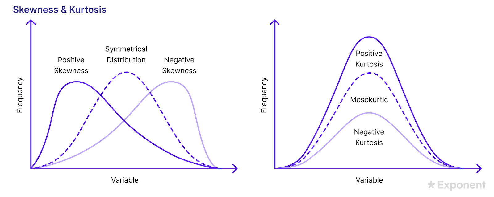
1. How do you measure skewness?

Skewness is a situation where data is not distributed symmetrically to the left and right of the median.

In such cases, the bell curve is skewed to the right or left.

A right-skewed distribution is longer on the right side while a left-skewed distribution is longer on the left side.

The data has zero-skewness if the graph is symmetrical.

The two methods for measuring skewness are Pearson’s first and second coefficients.

Pearson’s first coefficient of skewness is computed by subtracting the mode from the mean and dividing the difference by the standard deviation.

Subtracting the median from the mean, then multiplying by three and dividing the product by standard deviation yields Pearson’s second coefficient of skewness.

2. What are the types of sampling?

Sampling is a technique for creating a subset from a dataset or population to reduce the cost of collecting data from an entire population.

In simple random sampling, a subset is selected from a larger population at random, meaning that each member of the population has an equal chance of being selected.

Researchers love this method due to its simplicity and lack of bias.

For example, a researcher selects 100 students from a school by assigning each student a unique number and using a random number generator to select the sample.

Systematic sampling involves picking observations at regular intervals from a list or ordered population.

For example, a quality control manager selects every 5th item from a production line for inspection.

In stratified sampling, the population is divided into distinguishable subgroups known as strata depending on specific traits.

Samples are then drawn independently from each stratum to ensure that all the subgroups are represented.

For example, a market researcher can divide customers based on their location and select individuals randomly from each group for a survey.

3. Which imputation methods do you recommend for handling missing data?

There are several methods for handling missing values, including:

• Employing an algorithm that handles missing values
• Predicting the missing values
• Imputation using the mean, mode, or median
• Assign a unique value to the missing values
• Dropping rows with missing values

If the data is large enough and the missing values are small, deleting the missing rows will not add or remove bias.

On the other hand, using a method such as mean imputation can lead to misleading results because it doesn’t take into account the correlation between features and reduces the variance.

4. Explain mean, mode, and median.

Mean, mode and medium are measures of central tendency used by data scientists to summarize and understand data distributions.

The mean or average of a dataset is obtained by adding all the values and dividing by the total number of values in the dataset.

It is sensitive to outliers because it considers the magnitude of all values.

The median is the middle value in a dataset when all the values are sorted in ascending or descending order. The median is less sensitive to outliers compared to the mean.

The median is a better measure of central tendency when the distribution is skewed or when there are outliers.

The mode is the number that occurs most often in a dataset and can be used for both categorical and numerical data.

It is commonly used to identify the central tendency of categorical values.

5. What is selection bias? How can you avoid it?

Selection bias occurs when the chosen sample is not a good representation of the entire population due to inappropriate sampling criteria.

Selection bias can be avoided by using probability-based sampling methods such as random, systematic, cluster, and stratified sampling.

6. How do you identify outliers?

An outlier is an observation in a dataset that differs significantly from other data points by either being too low or too high.

Outliers should be identified and dealt with appropriately to prevent them from affecting the analysis.

One way to identify outliers is using the Interquartile Range (IQR), which is the difference between the third quartile and the first quartile.

An outlier is identified as values less than Q1-1.5IQR or greater than Q3 + 1.5IQR.

Outliers can also be identified using statistical tests such as z scores.

For example, a value of 200 in an age column is an outlier and should be removed to prevent skewing analysis and affecting the accuracy of a model.

7. What are the potential biases resulting from using sampled data?

Possible biases include sampling bias, survivorship bias, and under-coverage bias.

Sampling bias is caused by non-random sampling, survivorship bias involves focusing on entities that passed a selection process while ignoring those that did not, and under coverage sampling involves sampling too few observations.

8. Explain kurtosis.

As mentioned above, skewness is a situation where data is not distributed symmetrically to the left and right of the median.

In such cases, the bell curve is skewed to the right or left.

A right-skewed distribution is longer on the right side while a left-skewed distribution is longer on the left side. The data has zero-skewness if the graph is symmetrical.

An example of a right-skewed distribution is household income where there are many households with low income and a majority with low income.

If you surveyed people about their retirement age, you would get a right-skewed distribution because most people retire when they are 60 or older.

Kurtosis measures the tailedness of a distribution compared to a normal distribution.

A high kurtosis indicates the presence of outliers in the dataset which can be mitigated by either adding more data or removing the outliers.

A dataset with low kurtosis is light-tailed and is less prone to outliers.

Kurtosis is used as a measure of risk in finance.

A high kurtosis indicates the probability of extremely high or low returns while a low kurtosis indicates moderate risk where the probability of extreme returns is low.

9. Which are the common measures of variability in statistics?

Standard deviation, range, and variance are the common measures of variability in statistics.

• Standard deviation measures the dispersion of data points around the mean and is calculated as the square root of its variance. A larger standard deviation indicates greater variability while a smaller one indicates less variability.
• Variance is computed from the average of the squared deviations from the mean. The values from variance are much larger than those of standard deviation, hence the standard deviation is easier to interpret.
• Range measures the difference between the largest and smallest values in a dataset. A large range indicates greater variability while a smaller range indicates less variability.

10. Explain the types of missing data.

The main types of missing data are:

• Missing completely at random (MCAR)
• Missing at random (MAR)
• Missing not at random (MNAR)

In MCAR, the probability of data being missing is random and independent of any observed or unobserved variables in the dataset.

Since the missingness is not related to any observed data, rows with missing values can be deleted or imputed with simple methods such as mean or median to prevent the reduction of the sample size.

In MAR, the probability of a value being missing can be explained by another observed variable. The missingness doesn’t depend on the unobserved data but on some of the data in the dataset.

The missing values can be predicted from other variables in the dataset. Model-based imputation methods can be used to impute the missing values because they factor in the relationship between the values used to predict missing values.

In MNAR, the probability of data being missing depends on the missing values themselves and the unobserved values. Imputing MNAR values requires more advanced techniques such as pattern mixture models or selection models.

11. Discuss data scaling, standardization, and normalization.

Scaling, standardization, and normalization are data preprocessing techniques used for scaling and transforming data into a standard scale.

• Scaling involves setting all the values in a dataset to be within a certain range such as 0 and 1 or -1 and 1. This ensures that all the values are within the same magnitude for analysis and model training.
• Standardization transforms a dataset to have a mean of 0 and a standard deviation of 1. This makes the distribution of the dataset normal allowing algorithms to converge faster and perform better.
• Normalization rescales features to have a mean of 0 and a standard deviation of 1 without constraining the values with a specific range. This is important when the distribution of the data is not normal and has varying scales.

Probability & Regression Questions

Below, we explore some common probability and regression questions in data science interviews.

1. What is the Law of Large Numbers?

The law of large numbers (LLN) states that as the size of a sample increases, the average of the sample approaches the population mean.

This means that the average of many independent and identically distributed random variables tends to converge to the expected value of the underlying distribution.

The average of the results from a random experiment tends to the mean as the number of trials increases. The law is used to understand how random variables behave over many trials.

This ensures that the average results from many independent and identically distributed trials converge to the expected value.

You are more like to reach the true average in a statistical analysis by choosing 20 instead of 2 data points in a population of 100 items.

The chances of the 20 values being a true representation of the entire dataset are higher than when only 2 values are chosen. Therefore, you are more likely to reach the true population mean as you randomly sample 20 values compared to 2.

2. What is the central limit theorem?

The central limit theorem states that the sample mean approaches a normal distribution as the sample size gets larger regardless of the population distribution.

Therefore, you can study the statistical properties of any distribution if the sample is big enough.

The theorem is used in hypothesis testing and computing confidence intervals.

The following conditions must be met for the central limit theorem to hold:

• The samples should be independent of each other.
• The sample size should be at least 30
• The population samples should be picked randomly

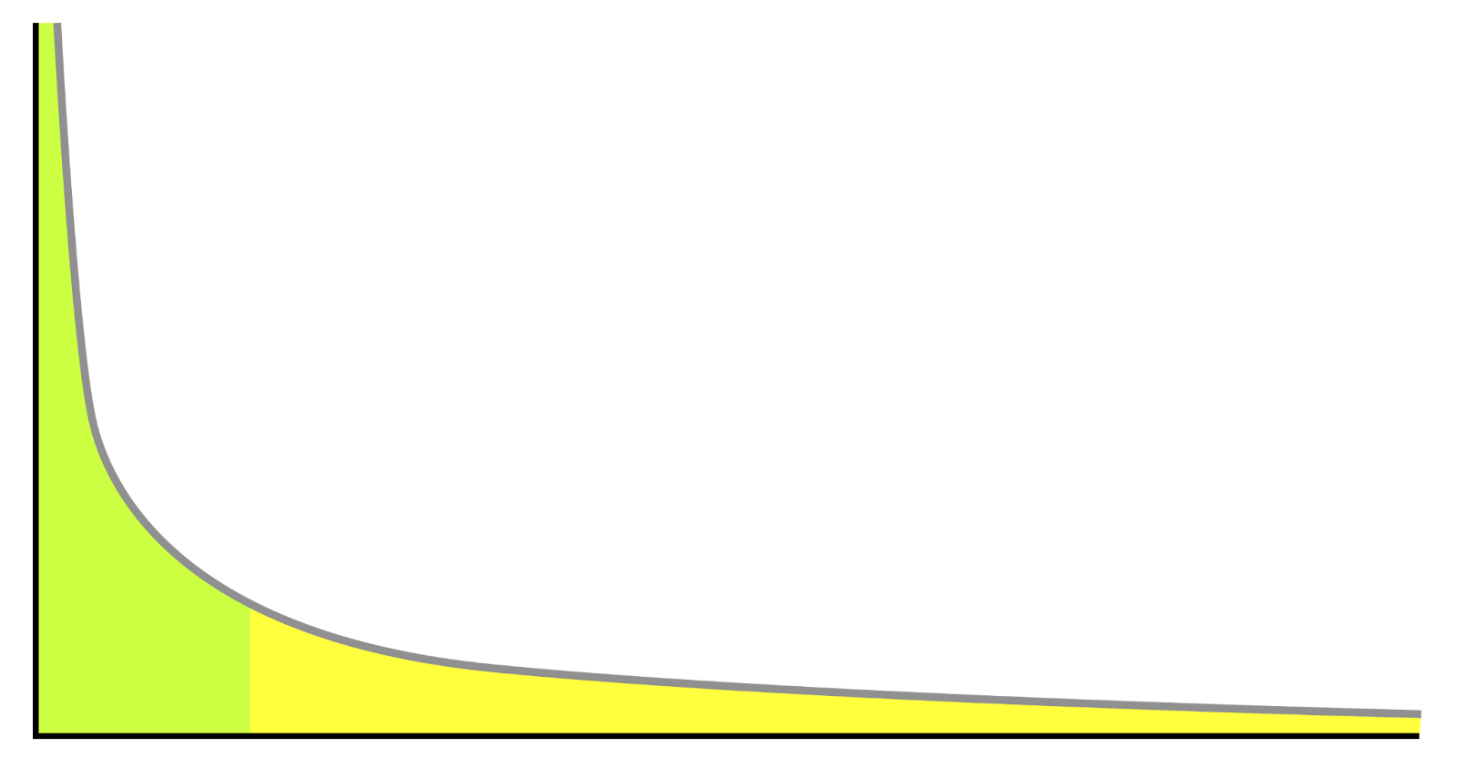
3. Explain long-tailed distributions and their significance in classification and regression problems.

In a long-tailed distribution, the tail of the curve decreases gradually as it approaches the end of the curve.

An example of a long-tailed distribution is book sales where the best sellers have the most sales while the majority of the books have a few sales.

In a business setting this can be an opportunity where a business can capitalize on getting a few sales from thousands of less popular books.

This phenomenon can affect the way you deal with outliers and the type of machine learning models that you apply to the dataset.

4. What are common assumptions of ordinary least squares?

Ordinary least squares (OLS) is a common technique for fitting a linear regression model to data aiming to find the line of best fit. The key assumptions of OLS are:

• The relationship between dependent and independent variables is linear.
• Independent variables are not highly correlated, preventing the model from learning the effect of each on the dependent variable.
• Errors are normally distributed especially for datasets with small sample sizes.
• The variance of the errors is constant for all independent variables.
• The errors or residuals are independent of each other, meaning that the error term for one data point can not predict the error term for another one.

5. What are common techniques for evaluating a model’s fit?

Various methods can be used to assess if a model fits the data, including:

• Root mean squared error (RMSE) for evaluating the deviation between predicted and true values in a regression model. Smaller values indicate a better fit.
• R-squared measures the proportion of the variation in the dependent variable that is predictable from the independent variables. The score lies between 0 and 1, with 1 meaning the model explains all the variability and 0 meaning that the model explains none of the variability. The value can be negative if the model is arbitrarily worse.
• Adjusted R-squared adjusts for the number of independent variables in the model. It prevents overfitting by penalizing the inclusion of unwanted features. Adjusted R-squared is lower than R-squared especially when there are many predictors in the model.

Hypothesis Testing & Confidence Interval Questions

Hypothesis testing and confidence intervals are key concepts in quantifying uncertainty and communicating the results to stakeholders. Here are some common hypothesis testing and confidence interval questions that you may encounter.

1. Explain Chi-square, ANOVA, and the t-test.

The Chi-Square Test is a statistical method for determining if two categorical variables are independent. For example, a food delivery startup can use Chi-square to determine the association between location and people’s food choices.

Analysis of Variance (ANOVA) is a statistical formula used to analyze variances across the means of different groups. The two main types of ANOVA are:

• One-way ANOVA involving a single independent variable.
• Two-way ANOVA involving two independent variables.

The t-test is used to compare the mean of two groups of normally distributed samples. The different types of t-tests include:

• One sample t-test that compares the mean of a sample and the population.
• Two sample t-tests for checking if the population of two independent samples is statistically different compared to the mean.
• Paired t-test for comparing the mean of different samples from the same group.

2. Discuss the null hypothesis and p-value.

The null hypothesis is the default hypothesis while the alternative hypothesis is the hypothesis that contradicts the null hypothesis. For example in the case of flipping a coin 10 times and observing one head, the null hypothesis is that the coin is fair. The alternate hypothesis is that the coin is not fair.

The p-value is used to check the evidence against the null hypothesis. The result is statistically significant if the p-value is smaller than the significance level. In that case, we reject the null hypothesis, otherwise, we fail to reject the null hypothesis.

3. What is the relationship between the significance level and the confidence level?

The significance level determines the amount of evidence required to reject the null hypothesis.

Common values are 0.05 (5%) and 0.01 (1%).

This means that accept a 5% or 1% probability of falsely rejecting the null hypothesis when it is true.

The confidence level is computed as 1 minus the significance level and is the probability of your estimates lying inside the confidence interval.

The confidence interval is the range of values that you expect your estimate to fall. For example, a confidence interval of 95% confidence level means that 95 out of 100 times, the estimate will fall within the confidence interval.

4. How do you determine statistical significance?

The statistical significance of an insight is determined by hypothesis testing.

It is done by creating a null and alternative hypothesis and then calculating the p-value.

Next, determine a significance level and reject the null hypothesis if the p-value is less than it. This means that the results are statistically significant.

5. How is root cause analysis different from correlation?

Root cause analysis is a problem-solving method that involves examining the root cause of a problem.

Correlation, a value between -1 and 1, measures the relationship between two variables. For example, a high crime rate in a town may be directly associated with high alcohol sales.

This means that they have a positive correlation but it doesn’t necessarily mean that one causes the other. Causation can be determined through hypothesis or A/B testing.

6. What are the differences between Type I and Type II errors?

Type I (false positive) happens when the null hypothesis is rejected when it’s true.

For example, a woman’s pregnancy test turns out positive when she is not pregnant.

Type II (false negative) happens when the null hypothesis is incorrectly not rejected when it is false.

For example, diagnosing a cancer test as negative when it is positive.

Experimentation

Experiments are a common way for companies to validate the launch of new features or improve existing ones.

Here are some common experimentation questions that you may come across.

1. What is A/B testing and where can it be applied?

A/B testing is a hypothesis testing technique for comparing two versions, a control, and a variant. It is commonly applied in marketing to improve user experience.

For example, designing two web pages and checking the one that leads to more conversions by showing different pages to two random samples of users.

2. In which situations are A/B tests not appropriate?

A/B tests aren’t appropriate:

• In scenarios with low traffic such as a low-traffic website which will take a long time to generate data.
• When the user behavior is complex and difficult to control, for example testing a new feature on repeat patients in a hospital system may be difficult because it’s not possible to predict when the patient will visit that specific hospital again, unless they have a chronic illness.
• When there are ethical constraints in running the A/B test and user consent is required.

3. Suppose a factory produces light bulbs, and two machines, A and B, are responsible for producing them. Machine A produces 60% of the bulbs. Machine B produces 40%. Machine A produces defective bulbs at a rate of 5%. Machine B produces defective bulbs at a rate of 3%. If a randomly selected bulb is defective, what is the probability that it was produced by machine A?

The problem is to determine the probability that a randomly selected bulb is defective and produced by machine A.

This requires the use of the Bayes theorem.

Our probabilities are:

• P(A) = Probability that Machine A produces the bulb = 60% = 0.6
• P(B) = Probability that Machine B produces the bulb = 40% = 0.4
• P(D) = Probability that a bulb is defective
• P(D|A) = Probability that a bulb is defective given it was produced by A = 5% = 0.05
• P(D|B) = Probability that a bulb is defective given it was produced by B = 3% = 0.03
• P(A|D) = Probability that a bulb produced by machine A is defective:
• Therefore, P(D) = P(D|A)P(A) + P(D|B)*P(B) = 0.050.6 + 0.030.4 = 0.042

Bayes theorem calculation:

• P(A|B)P(B) = P(B|A)P(A)
• Therefore, P(A|D) = P(D|A)*P(A)/P(D) = 0.05*0.6/0.042 = 5/7

Given a randomly selected bulb is defective, the probability that it is produced by Machine A is 5/7.

Interview Tips

It is impossible to cover all the possible questions since statistics is a vast subject.

Hopefully, these questions have given you a glimpse into what to expect in your data science interviews.

Explore dozens of mock interviews and practice lessons in our data science interview course.

Schedule a free mock interview session to practice answering questions with other peers.

Get data science interviewing coaching from scientists at top companies who have numerous years of experience.

Good luck with your upcoming interview!